Image2Mesh: a learning framework for single image 3D reconstruction
Abstract
A challenge that remains open in 3D deep learning is how to efficiently represent 3D data to feed deep neural networks. Recent works have been relying on volumetric or point cloud representations, but such approaches suffer from a number of issues such as computational complexity, unordered data, and lack of finer geometry. An efficient way to represent a 3D shape is through a polygon mesh as it encodes both shape’s geometric and topological information. However, the mesh’s data structure is an irregular graph (i.e. collection of vertices connected by edges to form polygonal faces) and it is not straightforward to integrate it into learning frameworks since every mesh is likely to have a different structure. Here we address this drawback by efficiently converting an unstructured 3D mesh into a regular and compact shape parametrization that is ready for machine learning applications. We developed a simple and lightweight learning framework able to reconstruct high-quality 3D meshes from a single image by using a compact representation that encodes a mesh using free-form deformation and sparse linear combination in a small dictionary of 3D models. In contrast to prior work, we do not rely on classical silhouette and landmark registration techniques to perform the 3D reconstruction. We extensively evaluated our method on synthetic and real-world datasets and found that it can efficiently and compactly reconstruct 3D objects while preserving its important geometrical aspects.

Overview
Given a single image, our framework employs a convolutional autoencoder to extract the image’s latent space, $\mathbf{z}$, that is used to classify it to an index, $c$, using a multi-label classifier and regress it to a compact shape parametrization using a feedforward network. We use a graph embedding, $\mathcal{G}$, that compactly represents 3D mesh objects to reconstruct the 3D model. Firstly, the estimated index, $c$, selects the closest 3D model to the image from the graph. Secondly, the selected model is deformed through the estimated parameters - free-form deformation (FFD), $\mathbf{\Delta P}$, and sparse linear combination parameters (i.e. $\alpha$’s). In this example, model 1 is selected (arrows 1 and 2), FFD is then applied (arrows 3 and 4), and finally the linear combination with the nodes 3, 4, 5, 6, and 7 (blue arrows on the graph that indicates the models in dense correspondence with node 1) are performed (arrow 5) to reconstruct the final 3D mesh model (arrow 6).
Results
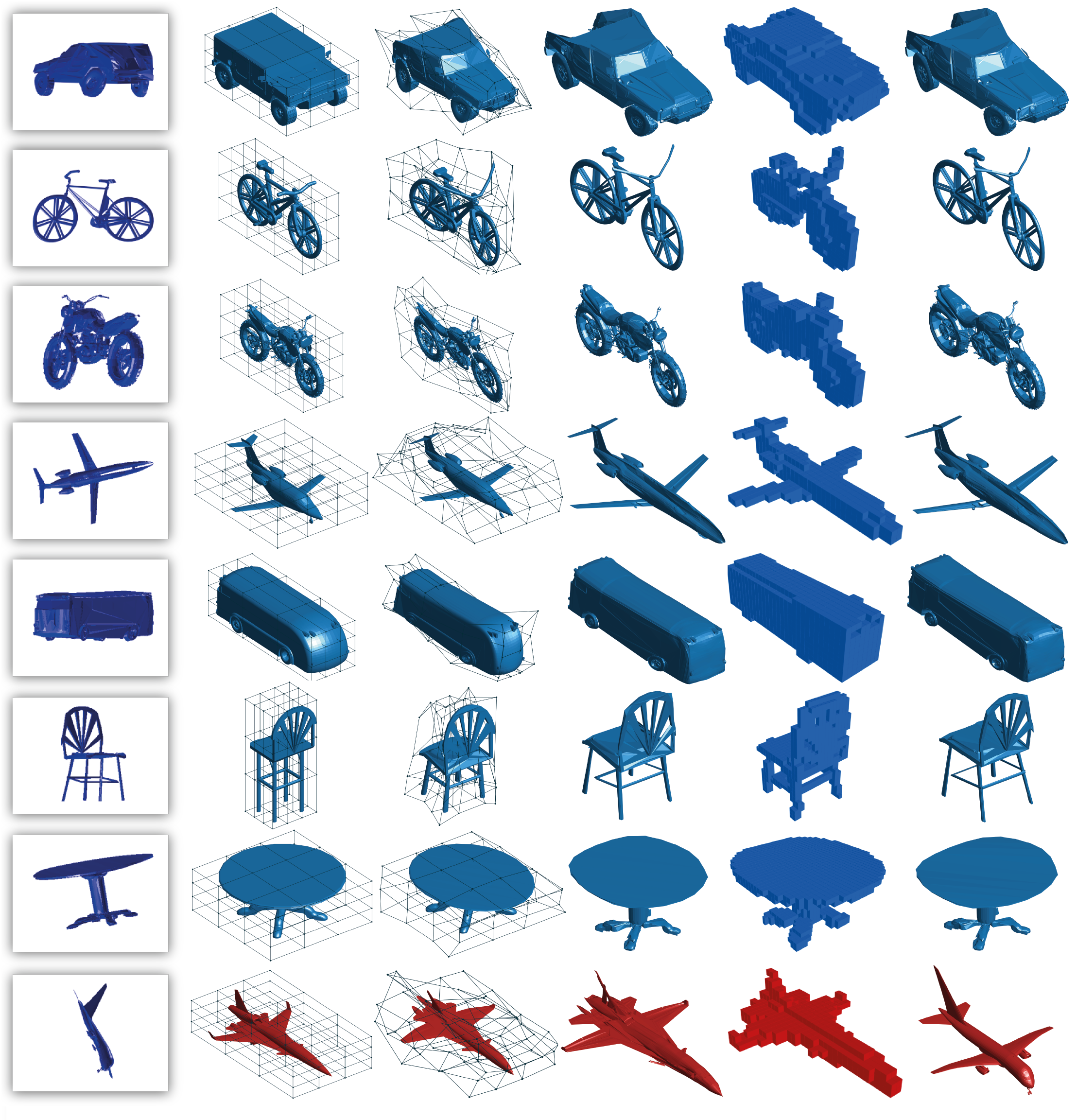
Qualitative results for the synthetic dataset. Column (a) shows the input image. Column (b) shows the selected model from the graph. Column (c ) shows the selected model with the FFD parameters applied. The final 3D model reconstructed by applying the linear combination parameters is shown in column (d) and the ground truth in (e).
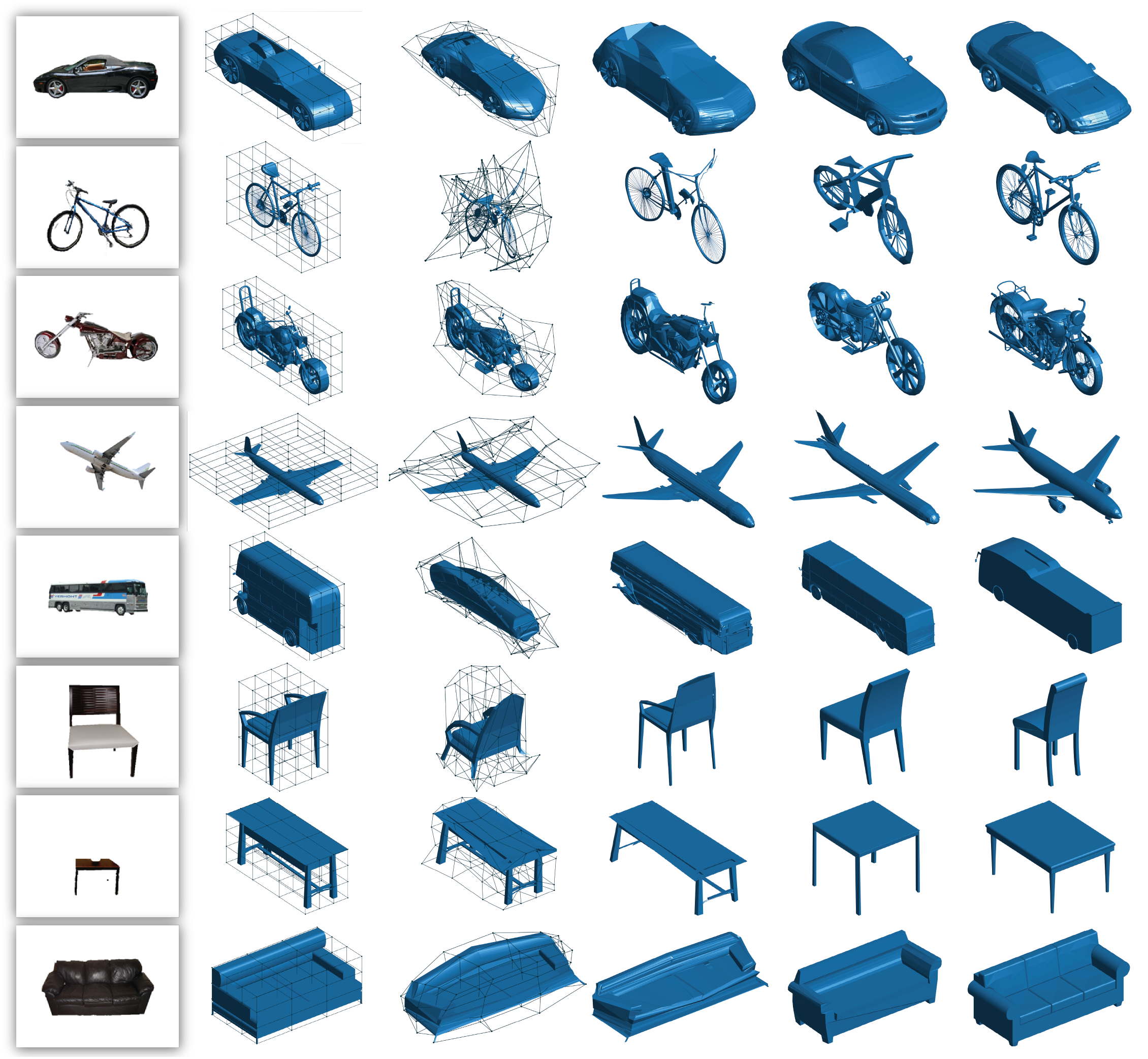
Qualitative results for the real-world dataset. Column (a) shows the input image. Column (b) shows the selected model. Column (c ) shows the selected model deformed by the FFD parameters. The final 3D model reconstructed by applying the linear combination parameters is shown in column (d). We compare with [18] in column (e) and the ground truth is shown in column (f).
A closer look at the 3D reconstruction.
More static examples
Qualitative results for the synthetic dataset. Column (a) shows the input image. Column (b) shows the selected model from the graph. Column (c ) shows the selected model with the FFD parameters applied. The final 3D model reconstructed by applying the linear combination parameters is shown in column (d). The voxelized final model is shown in column (e) and the ground truth in column (f). In the success cases (blues), one can see that the final models are similar to the ground truth with slightly differences that can be hard to point it out. A failure case is shown on the last row in red where a “wrong” model was selected from the graph.


Qualitative results for the real-world dataset. Column (a) shows the input image. Column (b) shows the selected model. Column (c ) shows the selected model deformed by the FFD parameters. The final 3D model reconstructed by applying the linear combination parameters is shown in column (d). We compare with [18] in column (e) and the ground truth is shown in column (f).


Please check the supplementary material out for more examples.