Abstract
Before the deep learning revolution, many perception algorithms were based on runtime optimization in conjunction with a strong prior/regularization penalty. A prime example of this in computer vision is optical and scene flow. Supervised learning has largely displaced the need for explicit regularization. Instead, they rely on large amounts of labeled data to capture prior statistics, which are not always readily available for many problems. Although optimization is employed to learn the neural network, the weights of this network are frozen at runtime. As a result, these learning solutions are domain-specific and do not generalize well to other statistically different scenarios. This paper revisits the scene flow problem that relies predominantly on runtime optimization and strong regularization. A central innovation here is the inclusion of a neural scene flow prior, which uses the architecture of neural networks as a new type of implicit regularizer. Unlike learning-based scene flow methods, optimization occurs at runtime, and our approach needs no offline datasets—making it ideal for deployment in new environments such as autonomous driving. We show that an architecture based exclusively on multilayer perceptrons (MLPs) can be used as a scene flow prior. Our method attains competitive—if not better—results on scene flow benchmarks. Also, our neural prior’s implicit and continuous scene flow representation allows us to estimate dense long-term correspondences across a sequence of point clouds. The dense motion information is represented by scene flow fields where points can be propagated through time by integrating motion vectors. We demonstrate such a capability by accumulating a sequence of lidar point clouds.
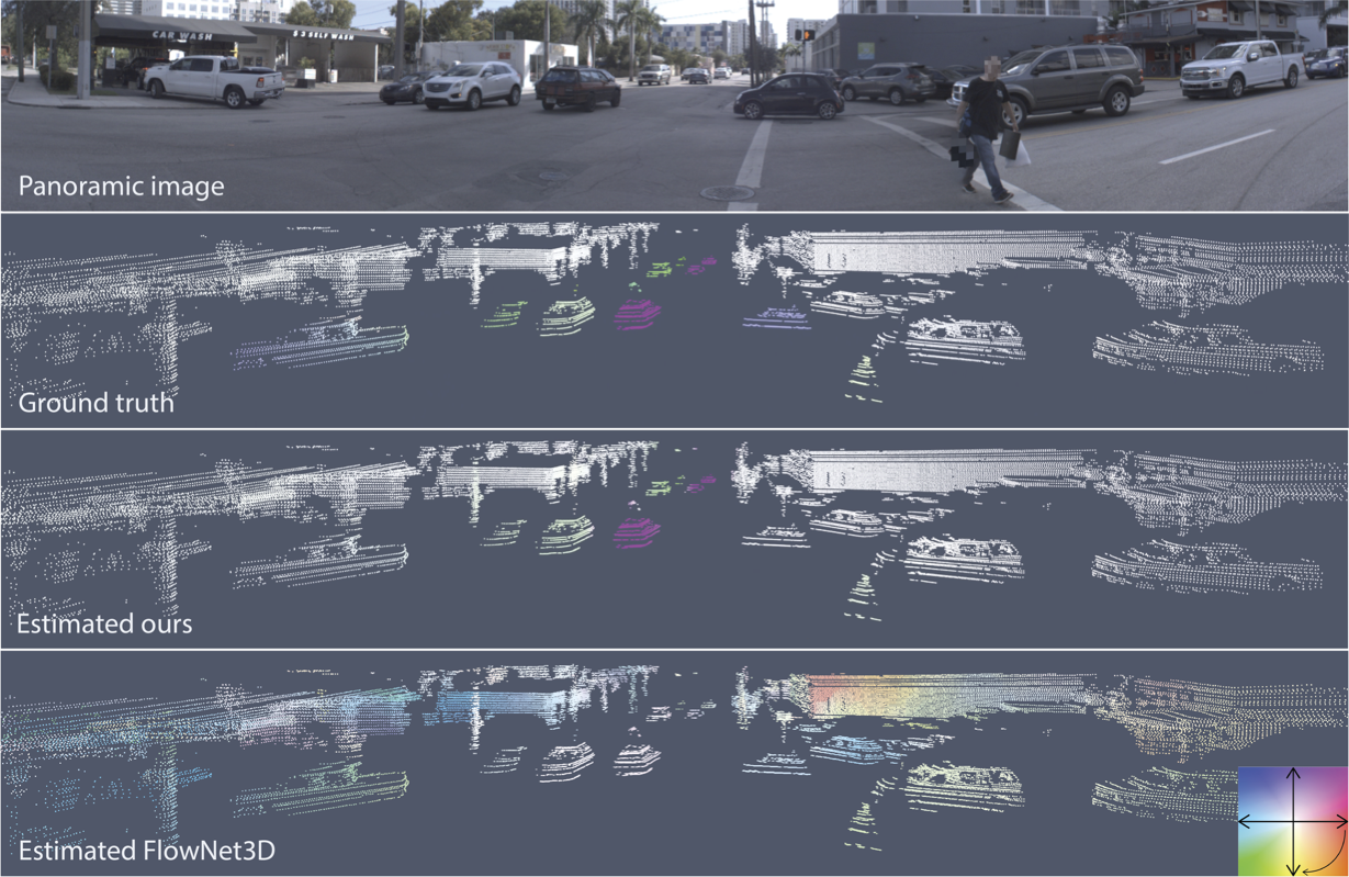 Qualitative example of a scene flow estimation using our proposed method. The complex and highly dynamic driving scene is from the Argoverse Scene Flow dataset. The scene flow estimated by our method is close to the ground truth. We also show a prediction using the supervised FlowNet3D method trained on FlyingThings3D and fine-tuned on the KITTI Scene Flow dataset. Note how the scene flow deviated from the ground truth when the inference was performed on an out-of-the-distribution sample. The scene flow color encodes the magnitude (color intensity) and direction (angle) of the flow vectors. For example, the purplish vehicles are heading northeast.
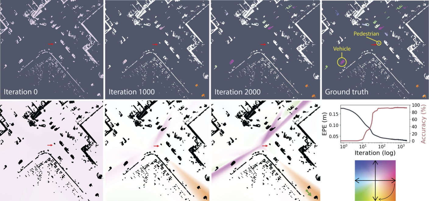 Example showing how the estimated scene flow and the continuous flow field (bottom) given by our neural prior change as the optimization converges to a solution. We show a top-view dynamic driving scene from Argoverse Scene Flow. The scene flow color encodes the magnitude (color intensity) and direction (angle) of the flow vectors. For example, the purplish vehicles are heading northeast. The red arrow shows the position and direction of travel of the autonomous vehicle, which is stopped, waiting for a pedestrian to cross the street. Note how the predicted scene flow is close to the ground truth at iteration 2k. At iteration 0, the scene flow is random, given the random initialization of the neural prior. Thus having very small magnitudes for the random directions. As the optimization went on, the flow fields became better constrained. A simple way to interpret the
flow fields is to imagine sampling a point at any location in the continuous scene flow field to recover an estimated flow vector. For example, imagine sampling a point around the orange region in the flow field at iteration 2k (green arrow in the bottom right). The direction of the flow vector will be pointing southeast at a specific magnitude, similar to the vehicles in the orange region.
Example showing how the estimated scene flow and the continuous flow field (bottom) given by our neural prior change as the optimization converges to a solution. We show a top-view dynamic driving scene from Argoverse Scene Flow. The scene flow color encodes the magnitude (color intensity) and direction (angle) of the flow vectors. For example, the purplish vehicles are heading northeast. The red arrow shows the position and direction of travel of the autonomous vehicle, which is stopped, waiting for a pedestrian to cross the street. Note how the predicted scene flow is close to the ground truth at iteration 2k. At iteration 0, the scene flow is random, given the random initialization of the neural prior. Thus having very small magnitudes for the random directions. As the optimization went on, the flow fields became better constrained. A simple way to interpret the
flow fields is to imagine sampling a point at any location in the continuous scene flow field to recover an estimated flow vector. For example, imagine sampling a point around the orange region in the flow field at iteration 2k (green arrow in the bottom right). The direction of the flow vector will be pointing southeast at a specific magnitude, similar to the vehicles in the orange region.
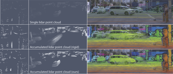 Example of a scene flow integration to densify an Argoverse lidar point cloud. The left and middle columns are a top and front view of the point cloud, respectively. The rightmost column shows the accumulated point cloud projected onto the image. Note the smearing effect on the dynamic objects when rigidly accumulating the point clouds (middle row). Accumulation using our neural prior nicely produced a denser point cloud while taking care of all dynamic objects in the scene. Here, rigid means that the point cloud accumulation was performed using a rigid registration method (i.e., ICP) where rigid 6-DoF poses are used for the registrations